Getting Started

In an earlier article I gave a quick overview of my first experiment with Tableau Public, in which I extracted data from the Environment Agency’s (EA’s) Bathing Water Quality data API via Tableau Public’s web data connector (WDC) mechanism. We also have an earlier article with some background on Bathing Water Quality that might give some useful context.

This series of posts continue the theme as I go into more detail about using Tableau, I also explore a few enhancements in the visualisation such as making the presentation and interaction richer, linking out to EA’s website and pulling in data Bathing Water Quality data from Wales and Scotland.

Part 1 | Part 2 | Part 3 | Part 4

Starting with CSV Data

The earlier article was based on my first experiment with Tableau Public. It was motivated by i) wanting to try out Tableau Public and ii) the idea that by using a live API (Application Programming Interface) as the data source in Tableau Public, I would be able to configure the hosted visualisation to update each time a user visited it – so would always provide up-to-date data.

As I expain in Part 4 of this series, I was mistaken in that – once it is imported via the API, the data in the public/hosted visualisation is static – i.e. it can’t be configured to update every time a user visits the dashboard page.

Given that the Bathing Water Quality data API can provide the data in CSV (Comma-Separated Value) format – the stardard open spreadsheet format – and Tableau Public can import CSV files directly (no need for creating a Web Data Connector). In the this post I’ll briefly describe the process of creating the original Dashboard, but using a CSV from the API rather than the Web Data Connector.

In the original experiment I used the API to get json. The URL used was:

https://environment.data.gov.uk/doc/bathing-water.json?_view=bathing-water&_pageSize=1000&_page=0

The retured json file [see example at the end of this post] contains all of the key data about designated bathing waters in England, including:

Name name
Bathing Water ID eubwid notation
Latitude and Longitude sampling point > lat, sampling point > long
Latest annual water quality classification latest compliance assessment
Local Authority area district
Water Company area appointed sewerage undertaker

Getting the CSV Data

To get it as a CSV we can simply replace the json in the url with csv.

https://environment.data.gov.uk/doc/bathing-water.csv?_view=bathing-water&_pageSize=1000&_page=0

The CSV file also includes columns for uri (Uniform Resource Identifier) for the things the data is about (bathing water, classification, etc.). Those identifiers are web URLs that can be used to link to web-pages containing data about those things – a valuable feature of linked data.

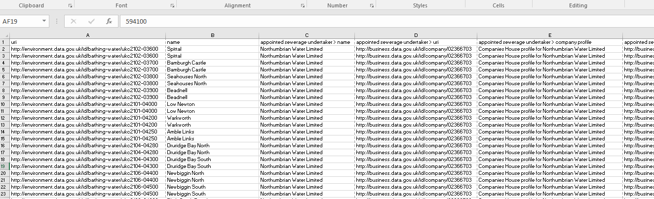
Important note: the CSV will contain two rows per bathing water that’s because the underlying data provides two different values for district (local authority) identifiers. One linking to Ordnance Survey identifiers/linked data and one to the Office of National Statistics identifiers. There are also two bathing water ‘type’ values, one the general type, i.e. Bathing Water and one more specific, e.g. TransitionalBathingWater.

That’s a common situation, for many kinds of data there might be many values of a property rather than just two. The json formatted data can have multiple values for a property nested together, but CSVs have to flatten those out, so one solution is to create a row per different value of the particular property with all the other columns identical. Tableau Public can also import json files directly – although it is less straight forward than the csv – when used with the bathing water quality API’s json file, it too creates two data rows per bathing water.

It’s not a problem as we can use Tableau’s filters feature to tidy the data up just to include what’s required.

Creating the Dashboard(s)

Steps in creating the dashboard:

A. Download the Tableau Public App (current version Feb 2017 Tableau 10.1.4)

Creating Tableau Public visualisations/dashboards is done via the Tableau Public desktop application, so you will need to be able to install it on your computer to create them.

In most corporate IT environments, it’s likely you will need to talk to your IT department before installing the desktop application. It’s probably a good idea to check with them in any case.

B. Import the Data & Tidy It Up

Under connect to a file in the left hand side of the main screen, choose text file, that opens a file dialogue box, navigate to and select the file and click open.

The file will be imported – the data will appear as a table of columns in the bottom right pane of the window.

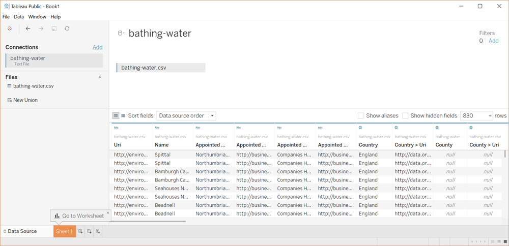
As noted above – at this point each Bathing Water has two rows. You can see there are a few differences between the two rows i) the district and ii) district > URI columns and iii) type > URI . We want to use the rows with named districts and don’t plan to use the type.

So we can filter rows where the district values are not Null (empty).

We can do that using Tableau’s filters– link top left of the window

There are also the unwanted uri columns, it will be helpful to hide those.

Roll over the Abc text at the top of the column and then click on the down arrow that appears to the right. Choose hide for each of the columns with URI in it (and any others you don’t want to see when creating visualisations)

C. Create Individual Charts and Map

In Tableau terminology a dashboard is a collection of individual worksheets, one worksheet for each of the charts and map. So each chart, map, etc. needs to be created individually (very quick) and then combined in one (or more) dashboard.

There isn’t room here to go through the process of creating and configuring all of the charts and map in detail, but there are many resources e.g. Tableau’s own, user forums and wider web resources/tutorials. I’ll show how to create a the district chart and map.

Creating each chart or map is mostly a matter of dragging and dropping – at least to get started. There are lots of configuration options once the basic choice are made.

Create the district bar chart:

click on the Sheet 1 tab at the bottom of the window
drag district from the list of dimensions to the vertical axis of the sheet or to the row box at the top of the window
drag number of records in the measures pane, to the columns box at the top of the window

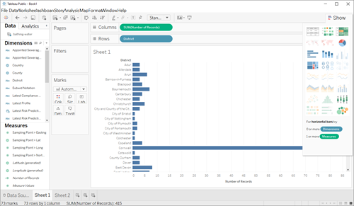
Rolling over a bar will bring up a box showing district name and a count of bathing waters in that district (i.e. with their district having that value.) Clicking on a bar will select that bar (and the bathing waters in that district), you will get the option to filter (keep only or exclude those bathing waters). If you do the bar chart will be updated to only show that bar or exclude it from the chart. That will show up in the filters box to the left of the chart – to remove a filter drag it out of that box.

To create the bathing water sampling point map:

This is a bit more complicated as we need to do some tidying up – but not much. Tableau makes some initial guesses when it brings data in.

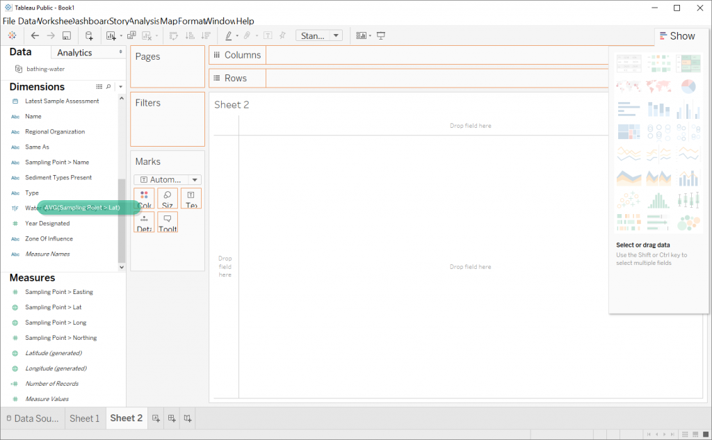
open a new worksheet – click on the New Worksheet icon to the right of the Sheet 1 at the bottom of the window
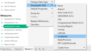
the Sampling Point > long is currently marked as a number, see the # symbol to the left of the name. The globe next to Sampling Point > lat shows its recognised as geographical data. We need to tell Tableau that the Sampling Point > long is geographical data and it is a longitude. See the figure below
the Sampling Point > lat and Sampling Point > long are initially measures (numbers to be counted, averaged, etc.), which was Tableau’s best guess. They need to be made into dimensions. Simply drag them one at a time to the dimensions pane
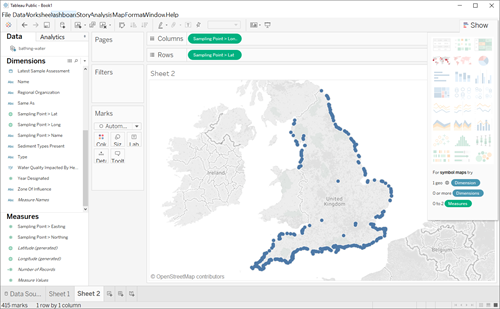
drag Sampling Point > lat to the row box at the top of the window and Sampling Point > long to the column box. Tableau automatically generates the map with dots to show the locations.

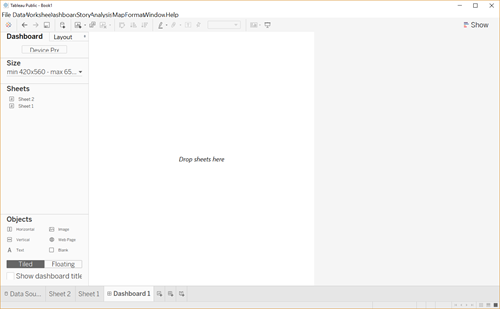
D. Create a Simple Dashboard:

click on the New Dashboard icon next to the New Worksheet icon at the bottom of the screen.
drag Sheet 1 from the Sheets pane to the left onto the blank dashboard canvas
drag Sheet 2 onto the lower half of the Sheets pane, the Sheet 1 chart should resize to only take up the top half with the map on the lower half. Now we can join the chart and map so that they act as filters to each other:
click on the Sheet 1 chart. Click on the funnel icon at the top right of the chart boarder – see figure below.

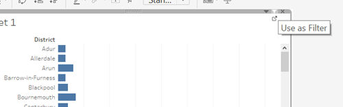
This will make the chart act as a filter for the other Sheets on the dashboard.

do the same for the map/Sheet 2.

The charts can now be used to filter each other, e.g. click on the Bournemouth bar on Sheet 1. The map will zoom to show the bathing waters in the Bournemouth district.

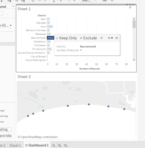
Clicking in the white space in Chart 1 or clicking again on the Bournmouth bar, will clear the filter.

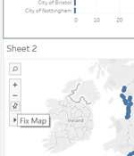
You can prevent the map from zooming by clicking on the pin icon that appears on the map controller when you roll over the map.

E. Saving the visualisation

When saving (via File>Save To Tableau Public…) it is only possible to save to Tableau Public’s servers that means that the visualisation will be public. There isn’t an option to have private or restricted visualisations.

Going Further With Charts and Dashboards

That gives a very basic illustration of how the charts and map were made. After writing the previous article I played with the various options and added some other features as other experiments. For example:

Experiment 1b

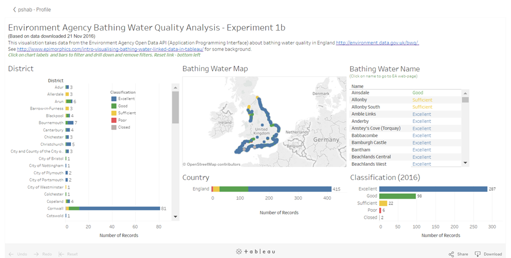
removed the water company chart and replaced it with a list of individual bathing water names, so that when filters were applied the bathing waters could be seen
added numbers to the chart columns so that they could be seen more easily
added external web-links from each item in that list of bathing waters to the EA’s bathing water profile page for each bathing water – that’s via the Tableau actions feature
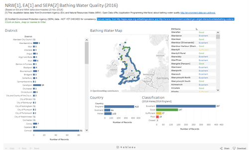
added classification as a colour dimension to all of the charts so that for each district, point on the map, etc. the water quality classification can be seen by colour
added a country chart so that the total number of bathing waters was clear

Adding in Welsh and Scottish Data

I was keen to add the Natural Resources Wales (NRW) Welsh bathing water data to the visualisation. The NRW use an API very similar to the Environment Agency’s – the NRW’s was also developed by Epimorphics.

In fact, in this case, I used exactly the same form of API call to get the Welsh data but with a different path.

https://environment.data.gov.uk/wales/bathing-waters/doc/bathing-water.csv?_view=bathing-water&_pageSize=1000&_page=0

I combined all of the data into a single spreadsheet – adding the Welsh data as rows to the English data (ensuring columns lined up) and saving it as a new spreadsheet. Replacing the original spreadsheet as the source in the Tableau Public application created a version including the Welsh data.

Finally I gathered the Scottish data – while the data is available as open data and via an interactive interface, I couldn’t find the data in a downloadable form or via an API. However I could pull it together from various sources, It was derived mainly from SEPA’s Bathing Waters Pages and Scotland’s Environment get interactive site about bathing waters.

Combining that with the English and Welsh data in a single new spreadsheet then led to a couple of other dashboards that combined the three country’s data:

Example of part of the json data (object) returned by the API

This section is about a bathing water Spittal returned by the API call use above.

{
"_about": "http:\/\/environment.data.gov.uk\/id\/bathing-water\/ukc2102-03600",
"appointedSewerageUndertaker": {
  "_about": "http:\/\/business.data.gov.uk\/id\/company\/02366703",
  "companyProfile": {
    "_about": "http:\/\/business.data.gov.uk\/companies\/profile\/02366703",
    "label": [
      {
        "_value": "Companies House profile for Northumbrian Water Limited",
        "_lang": "en"
      }
    ]
  },
  "name": {
    "_value": "Northumbrian Water Limited",
    "_lang": "en"
  }
},
"country": {
  "_about": "http:\/\/data.ordnancesurvey.co.uk\/id\/country\/england",
  "name": {
    "_value": "England",
    "_lang": "en"
  }
},
"district": [
  {
    "_about": "http:\/\/data.ordnancesurvey.co.uk\/id\/7000000000043674",
    "name": {
      "_value": "Northumberland",
      "_lang": "en"
    }
  },
  "http:\/\/statistics.data.gov.uk\/id\/statistical-geography\/E06000048"
],
"envelope": {
  "_about": "http:\/\/location.data.gov.uk\/so\/common\/Envelope\/bwpf.eaew\/ukc2102-03600:1",
  "label": [
    {
      "_value": "Map bounds for Spittal",
      "_lang": "en"
    }
  ]
},
"eubwidNotation": "ukc2102-03600",
"latestComplianceAssessment": {
  "_about": "http:\/\/environment.data.gov.uk\/data\/bathing-water-quality\/compliance-rBWD\/point\/03600\/year\/2016",
  "complianceClassification": {
    "_about": "http:\/\/environment.data.gov.uk\/def\/bwq-cc-2015\/3",
    "name": {
      "_value": "Sufficient",
      "_lang": "en"
    }
  }
},
"latestProfile": "http:\/\/environment.data.gov.uk\/data\/bathing-water-profile\/ukc2102-03600\/2016:1",
"latestRiskPrediction": {
  "_about": "http:\/\/environment.data.gov.uk\/data\/bathing-water-quality\/stp-risk-prediction\/point\/03600\/date\/20160930-083517",
  "expiresAt": {
    "_value": "2016-10-01T08:29:00",
    "_datatype": "dateTime"
  },
  "riskLevel": {
    "_about": "http:\/\/environment.data.gov.uk\/def\/bwq-stp\/normal",
    "name": {
      "_value": "normal",
      "_lang": "en"
    }
  }
},
"latestSampleAssessment": "http:\/\/environment.data.gov.uk\/data\/bathing-water-quality\/in-season\/sample\/point\/03600\/date\/20160919\/time\/100100\/recordDate\/20160919",
"name": {
  "_value": "Spittal",
  "_lang": "en"
},
"regionalOrganization": {
  "_about": "http:\/\/reference.data.gov.uk\/id\/public-body\/environment-agency\/unit\/north-east-north-east-office",
  "name": {
    "_value": "North East",
    "_lang": "en"
  }
},
"sameAs": "http:\/\/environment.data.gov.uk\/id\/bathing-water\/spittal",
"samplingPoint": {
  "_about": "http:\/\/location.data.gov.uk\/so\/ef\/SamplingPoint\/bwsp.eaew\/03600",
  "easting": 400800,
  "lat": 55.75686834582,
  "long": -1.9888393795735,
  "name": {
    "_value": "Sampling point at Spittal",
    "_lang": "en"
  },
  "northing": 651500
},
"sedimentTypesPresent": "http:\/\/environment.data.gov.uk\/def\/bathing-water\/sand-sediment",
"type": [
  "http:\/\/environment.data.gov.uk\/def\/bathing-water\/BathingWater",
  "http:\/\/environment.data.gov.uk\/def\/bathing-water\/CoastalBathingWater"
],
"uriSet": {
  "_about": "http:\/\/environment.data.gov.uk\/id\/bathing-water\/",
  "label": [
    {
      "_value": "Bathing waters monitored by the Environment Agency for England and Wales.",
      "_lang": "en"
    }
  ]
},
"waterQualityImpactedByHeavyRain": true,
"yearDesignated": "http:\/\/reference.data.gov.uk\/id\/year\/1988",
"zoneOfInfluence": {
  "_about": "http:\/\/location.data.gov.uk\/so\/ef\/ZoneOfInfluence\/bwzoi.eaew\/ukc2102-03600:1",
  "name": {
    "_value": "Zone of influence at Spittal",
    "_lang": "en"
  }
}
}

For more in this #TechTalk series see: Part 1 | Part 2 | Part 3 | Part 4